4. Flux

1 Quantitative Prediction of High-Energy Electron Integral Flux at Geostationary Orbit Based on Deep Learning

Wei, L., Zhong, Q., Lin, R., Wang, J., Liu, S., & Cao, Y. (2018). Quantitative prediction of high-energy electron integral flux at geostationary orbit based on deep learning. Space Weather, 16, 903–916. https://doi.org/10.1029/2018SW001829

1.1 简介

1.1.1 recurrent neural network (RNN)

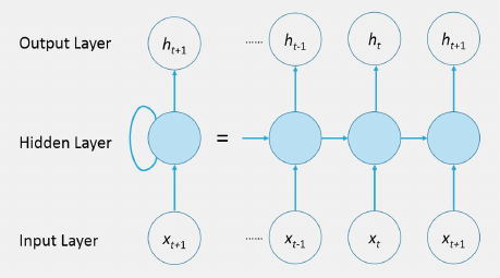
Unlike traditional feed-forward neural networks, RNNs add loops in themselves, allowing information to be retained from a previous time to the next by iterative function loops
The back-propagation trough time algorithm is used to adjust and renew the network parameters during the training process (residual calculation).
equation:

h_{t} = σ (W_{x h} x_{t} + W_{h h} h_{t - 1} + b)

a gradient vanishing and explosion problem exists if the input sequence is too long

1.1.2 Long Short-Term Memory (LSTM)

LSTM repeating module architecture	Meaning	Formulas
!401	$x_{t}$ : Input at moment $t$ $h_{t}$ : Output $C_{t}$ : Cell state ${\tilde{C}}_{t}$ : Candidate values $f_{t}$ : Forget gate function $i_{t}$ : Input gate function $o_{t}$ : Output gate function $σ, \tanh$ : Activation function Blue circles: Neural network layers $\times$ : Element-wise Multiplication ' $*$ '	$$\begin{array}c\begin{array}c f_t = \sigma(W_f \cdot [h_{t-1},x_t] + b_f)\ i_t = \sigma(W_i\cdot [h_{t-1},x_t] + b_i) \ \widetilde{C}t = \tanh(W_c\cdot [h,x_t] + b_C) \ C_t = f_t * C_{t-1} + i_t * \widetilde{C}_t \ o_t = \sigma(W_o \cdot [h_t-1,x_t] + b_o) \ h_t = o_t * \tanh(C_t) \end{array} \[8pt] \begin{cases} \sigma(x) = \frac{1}{1+e^{-x}} \[3pt] \tanh(x) = \frac{{1-e^{-2x}}}{1+e^{-2x}} \end{cases}\end{array}$$

LSTM layer principle ex.

Data Structure and Batch Processing
For time series [1,2,3,4,5], splitting to X=[[1,2],[2,3],[3,4],[4,5]] and y=[3,4,5,6]:

X contains 4 samples (batch_size=4), each sample is a sequence of length 2(time_step=2), and input_size=1 for 1D data series
The model processes these samples in batches, performing forward propagation independently for each sample
Taking the first sample [1, 2] as an example, the LSTM processing steps:
1. Time step 1: Process input 1, update hidden state h1
2. Time step 2: Process input 2, combine with h1 to update hidden state h2
3. Extract features: Take the hidden state from the last time step h2
4. Prediction: Map h2 to a predicted value through a linear layer, compare with target value 3

Parallelism in Batch Processing

The model processes multiple samples simultaneously (depending on batch_size)
For all 4 samples in X, the LSTM executes the above processing steps in parallel
The processing of each sample is independent, and ultimately each sample yields a predicted value

1.1.3 Calibration

The logarithm of the daily electron integral flux from the three pairs of GOES satellites during the overlapped period has strong. linear correlations. Based on this, the values from different satellites are calibrated using the data of GOES-11 by using the method of linear fitting that covers the time period from January 1999 to December 2016.

In addition, piecewise linear fitting is used to calibrate the data from GOES-13 to GOES-11.

1.1.4 Model Result

Spearman’s rank correlation analysis

Unlike the more common Pearson correlation, which looks for linear relationships (straight lines), Spearman looks for monotonic relationships. This means it checks if, as one variable increases, the other tends to increase (corr>0) or decrease(corr<0), even if that change isn't a perfectly straight line.

For a dataset without many tied ranks, the formula is:

r_{s} = 1 - \frac{6 \sum d_{i}^{2}}{n (n^{2} - 1)} = 1 - \frac{2 \sum d_{i}^{2}}{\sum i^{2}} \in [- 1, 1]

$d_{i}$ is the difference between the ranks of each observation.
$n$ is the number of observations.

How to Calculate it in Python:

# Offset Time: Shifting 'sales' back by 2 periods
df['sales_lagged'] = df['sales'].shift(-2)

# Using scipy
from scipy import stats
x = [10, 20, 30, 40, 50]
y = [2, 2.4, 10, 8, 25]
coef, p_value = stats.spearmanr(x, y)
print(f"Spearman Correlation Coefficient: {coef:.3f}")
print(f"P-value: {p_value:.3f}")

# Using pandas for DataFrame
import pandas as pd
df = pd.DataFrame({'study_hours': [1, 5, 2, 8, 4], 'test_scores': [50, 88, 60, 95, 78]})
correlation_matrix = df.corr(method='spearman')
print(correlation_matrix)

result:
!696
According to the correlation, the ﬂux itself, solar wind velocity, Dst, and Kp indices are considered to be better input factors for modeling. The remaining parameters, with the exception of IMF, are also used as inputs for modeling.

The feature of offset time is an important factor of setting the time step in modeling to determine the number of consecutive days to be used as inputs to the model.

1.1.5 Daily-Based Model

1.1.6 Hourly-Based Model

1.2 补充

_Documents/words/Part.4 words#1 Quantitative Prediction of High-Energy Electron Integral Flux at Geostationary Orbit Based on Deep Learning

1.3 链接

本地 4.1 Wei et al. - 2018 - Quantitative Prediction of High-Energy Electron Integral Flux at Geostationary Orbit Based on Deep Learning